ZenithSync Assay Planner
What should an experiment measure next?

Two plates, one curve, and three wells worth buying.
An illustration built for this site in Blender. It explains the idea; it is not data from the project.
Every measurement uses part of an experiment’s budget. Given one control and the lowest and highest doses already measured, which few wells should a lab buy next to pin down a drug’s dose-response curve? I built a planner that considers what is already known, where uncertainty remains, and how a shared control affects several treatment measurements at once.
The shared-control problem
A treatment response is read against a measured control. When several responses share that reference, their errors are related: if the control reads high, every contrast reads low together. The planner keeps this dependence instead of treating the control as perfectly known, and it can choose to buy another control well when that helps more than another treatment well.
A curve that starts at zero
The response is modelled as a Gaussian process over log dose, with a kernel adjusted so that the drug effect at zero dose is exactly zero. A control therefore carries no drug effect but still carries information, through the shared noise. Hyperparameters were chosen once by leave-one-organoid-out validation on a development dataset, where all 28 folds picked the same setting, and then frozen.
Choosing a batch exactly
For a fixed budget, the planner searches every possible set of wells and keeps the one that leaves the least average uncertainty across the planned doses. Wells that are interchangeable are grouped, so one representative stands for many equivalent sets: 13,408 representatives covered 2,113,536 subsets in the confirmation. A small counter-example in the tests shows why this matters: the best single well is not always part of the best pair.
Testing the claim on data it had not seen
The protocol was frozen and timestamped before the confirmation dataset’s responses were opened. That dataset has two parallel plates per context: wells are chosen from one and judged against the other. Across 6,496 contexts from 148 organoid samples and 100 patients, exact selection lowered mean squared error by 32.82% against random selection under the same model. Against the stronger greedy baseline the improvement was 0.66%, which is the honest size of the advantage of exact search.
What stayed in the record
On the development dataset the same comparison was inconclusive: every bootstrap interval included zero. An earlier liver-chip pilot gave no positive result either. Both remain in the repository beside the confirmation, along with a crashed first evaluator run that was preserved and amended for serialisation only.
The control well is part of the model.
- 01
Keep the covariance
Subtracting the same measured control from several treatment readings introduces shared error. With independent raw errors of variance s², the contrast-noise covariance is R = s²(I + 11ᵀ): 2s² on the diagonal and s² off it. The joint Gaussian model preserves that dependence; its error was 11.36% lower than an ablation that ignores it.
- 02
Search the finite design space
The optimizer chooses a fixed-budget batch by minimising the equally weighted posterior variance at the designed doses, C − C[:,A] C[A,A]⁻¹ C[A,:]. Verified exchangeable wells are grouped so one representative per count pattern is evaluated. This reduces enumeration without changing the optimum of the bounded problem, and it is checked against brute force in the tests.
- 03
Freeze, then evaluate
Model choices were fixed before confirmation on a separate public organoid study. Exact, greedy and random policies share the same prediction model and measurement budget. Inference resamples whole patients after averaging contexts within samples and samples within patients, so repeated contexts are not counted as independent evidence.
The covariance objective depends on the design and observed-well locations, not the response values. This is a fixed-model batch design; predictions update with measurements, but the selection rule is not response-adaptive. The endpoint is the error of the raw log treatment-minus-control signal, not viability.
Read the mathematical and contribution auditThe honest edges.
- These are retrospective results on public data. Savings in a real laboratory have not been demonstrated.
- The nominal 90% intervals covered 98.05% of held-back readings, so they are conservative rather than well calibrated.
- No clinical benefit, peer review or competition placement is claimed. I was the only team member and the only reviewer.
A closer look.
Original project walkthrough with synthetic narration. Recorded during the review stage. Read the transcript ↗
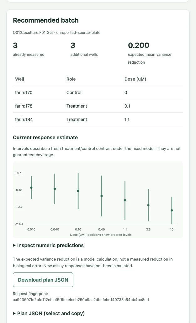
A plan you can inspect.
The local interface lists selected wells, their roles, and the model’s response estimates. The result can be downloaded for further inspection.
Project screenshot from the public research repository.
Where this connects.



These are retrospective research results. Prospective laboratory savings, clinical benefit, and transfer to perfused organ-on-a-chip experiments have not been demonstrated. Development data: Farin et al.; confirmation data: Kryeziu et al.; both public.